summar_A <- function(A, n = 3, func) {
  res <- list()
  for (i in 1:n) {
    a1 <- A[, grep(paste0("A\\[", i, ","), names(A))]
    a1_mean <- apply(a1, MARGIN = 2, func)
    res <- c(res, list(a1_mean))
  }
  res
}

summar_S <- function(S, n = 4, func) {
  res <- list()
  for (i in 1:n) {
    s1 <- S[, grep(paste0("S\\[", i, ","), names(S))]
    s1_mean <- apply(s1, MARGIN = 2, func)
    res <- c(res, list(s1_mean))
  }
  res
}

get_AS_hat <- function(A, S, estimate = "median", na = 15, ns = 4) {
  switch(
    estimate,
    median = list(
      A = summar_A(A, na, func = median),
      S = summar_S(S, ns, func = median)
    ),
    mode = list(
      A = summar_A(A, na, func = mode),
      S = summar_S(S, ns, func = mode)
    ),
    mean = list(
      A = summar_A(A, na, func = mean),
      S = summar_S(S, ns, func = mean)
    )
  )
}

scale_row_S <- function(row) {
  min_val <- min(row)
  max_val <- max(row)
  (row - min_val) / (max_val - min_val)
}

scale_row_A <- function(row) {
  row / sum(row)
}

mode <- function(x) {
  unique_x <- unique(x)
  unique_x[which.max(tabulate(match(x, unique_x)))]
}

get_plots_95_ci_spec <- function(p, S, func = "median", n = 2) {
  res <- list()
  for (i in 1:n) {
    s1 <- S[, grep(paste0("S\\[", i, ","), names(S))]
    s1_mean <- apply(s1, MARGIN = 2, func)
    s1_lower <- apply(s1, MARGIN = 2, function(x) quantile(x, probs = 0.025))
    s1_upper <- apply(s1, MARGIN = 2, function(x) quantile(x, probs = 0.975))
    res <- c(res, list(
      spectra = s1_mean,
      lower = s1_lower,
      upper = s1_upper
    ))
  }
  res
}

plot_95_ci_spec <- function(res, wavelength, spec_num) {
  i <- switch(as.character(spec_num),
              '1' = 1, '2' = 4, '3' = 7, '4' = 10)

  spectrum <- res[[i]]
  lower_bound <- res[[i+1]]
  upper_bound <- res[[i+2]]

  data <- data.frame(wavelength, spectrum, lower_bound, upper_bound)

  g1 <- ggplot(data, aes(x = wavelength)) +
    geom_ribbon(aes(ymin = lower_bound, ymax = upper_bound),
                fill = "red", alpha = 0.3) +
    geom_line(aes(y = spectrum), color = "blue", linewidth = 0.8) +
    theme_minimal() +
    labs(title = paste0("Median Spectrum ", spec_num, " with 95% CI"),
         x = "Raman Shift (index)",
         y = "Intensity")
  g1
}

get_A_values_and_median <- function(A, n = 2, func) {
  res <- list()
  for (i in 1:n) {
    a1 <- A[, grep(paste0("A\\[", i, ","), names(A))]
    a1_mean <- apply(a1, MARGIN = 2, func)
    res <- c(res, list("est" = a1_mean, "values" = a1))
  }
  res
}

get_plots_A_hist <- function(A_list, i) {
  dens <- density(A_list$values[, i])
  ci <- quantile(A_list$values[, i], probs = c(0.025, 0.975))

  dens_df <- data.frame(x = dens$x, y = dens$y)
  ci_df <- dens_df[dens_df$x >= ci[1] & dens_df$x <= ci[2], ]

  g1 <- ggplot() +
    geom_line(data = dens_df, aes(x = x, y = y), color = "blue") +
    geom_area(data = ci_df, aes(x = x, y = y), fill = "blue", alpha = 0.5) +
    geom_vline(xintercept = A_list$est[i], color = "red",
               linetype = "dashed", linewidth = 1) +
    theme_minimal() +
    labs(title = paste("Posterior Distribution of A[1,", i, "]"),
         x = "Value",
         y = "Density")

  return(g1)
}Bayesian Positive Source Separation for Raman Spectroscopy
Introduction
This notebook provides a walkthrough of my undergraduate honours thesis project in Bayesian Positive Source Separation (also known as Bayesian Nonnegative Matrix Factorization). Raman spectroscopy is an optical interrogation method capable of providing a unique “fingerprint” for both biological and non-biological compounds. However, the Raman spectra for a given chemical are actually a combination of the constituent spectra, thus, if we want to identify what chemicals are present, we require machine learning techniques to unmix the signal. This thesis combines group- and basis-restricted non-negative matrix factorization (GBR-NMF) (Shreeves et al. 2023) with Bayesian positive source separation (BPSS) (Brie et al. 2016) to create a probabilistic non-negative matrix factorization technique. Our method not only allows for the incorporation of prior knowledge, but also quantifies the uncertainty in the source separation process, an aspect missing from most standard NMF procedures. We use JAGS to perform Gibbs sampling for posterior inference.
The BPSS Model
Model Formulation
BPSS models the observed spectral data as a linear combination of pure component spectra with additive noise. The model is specified as:
\[\mathbf{X} = \mathbf{AS} + \mathbf{E}\]
where:
- \(\mathbf{X}_{m \times n}\) is the data matrix where each row vector represents a spectrum
- \(\mathbf{A}_{m \times p}\) is the mixing matrix with column vectors representing the mixing coefficients (concentrations) of each pure component
- \(\mathbf{S}_{p \times n}\) is the spectra matrix where each row vector is one of the \(p\) pure spectra
- \(\mathbf{E}_{m \times n}\) is the additive noise matrix
Prior Distributions
Noise Model
Each noise sequence (row vector of \(\mathbf{E}\)) is assumed to be independently and identically distributed Gaussian with zero mean and constant variance within a row:
\[p(\mathbf{E}|\theta_1)=\prod^m_{i=1}\prod^n_{k=1}\mathcal{N}(E_{(i,k)};0,\sigma^2_i)\]
where \(\theta_1 = [\sigma_1^2,\dots,\sigma_m^2]^T\).
Pure Spectra (S)
Each pure spectrum (row of \(\mathbf{S}\)) is assumed to follow a Gamma distribution with element-specific hyperparameters:
\[p(\mathbf{S}|\theta_2)=\prod^p_{j=1}\prod^n_{k=1}\mathcal{G}(S_{(j,k)};\alpha_j,\beta_j)\]
where \(\theta_2 = [\alpha_1,\dots,\alpha_p,\beta_1,\dots,\beta_p]^T\).
Mixing Matrix (A)
Each element of the mixing matrix is assumed to follow an Exponential distribution with element-specific rate parameters:
\[p(\mathbf{A}|\theta_3)=\prod^m_{i=1}\prod^p_{j=1}\text{Exp}(A_{(i,j)};\lambda_{i,j})\]
where \(\theta_3=[\lambda_{1,1},\dots,\lambda_{m,p}]^T\).
Hyperparameters
The prior for the precision of the noise is \(\mathcal{G}(2,\epsilon)\) assigned to \(\frac{1}{\sigma^2_i}\) where \(\epsilon\) is a small number (e.g., \(10^{-3}\)). The hyperparameters of \(\mathbf{S}\) follow \(\mathcal{G}(2,\epsilon)\) priors. The rate parameters \(\lambda_{i,j}\) of the Exponential distribution for \(\mathbf{A}\) also follow \(\mathcal{G}(2,\epsilon)\) priors.
Likelihood
The likelihood of the model is:
\[p(\mathbf{X}|\mathbf{S},\mathbf{A},\theta_1)\propto \prod^m_{i=1}\prod^n_{k=1}\left(\frac{1}{\sigma_i}\right)^n\exp \left[ -\frac{1}{2\sigma_i^2}\left(X_{(i,k)}-[\mathbf{AS}]_{(i,k)}\right)^2\right]\]
Helper Functions
These functions allow us to report 95% credible intervals and median point estimates for our model.
JAGS Model Specification
We use a Gamma-Exponential BPSS model where the pure spectra matrix S follows an Exponential distribution and the mixing matrix A follows a Gamma distribution:
BPSS_Gamma_Exponential <- "
model {
    for (i in 1:m) {
        for (k in 1:n) {
            X[i, k] ~ dnorm(mu[i, k], tau[i])
            mu[i, k] <- inprod(A[i, ], S[, k])
        }
    }

    for (j in 1:p) {
        for (k in 1:n) {
            S[j, k] ~ dexp(lambda_s[j,k]) T(0.001,1.001)
        }
    }

    for (i in 1:m) {
      for (j in 1:p) {
        A[i, j] ~ dgamma(alpha_a[i,j], beta_a[i,j]) T(0.001, 1.001)
      }
    }

    for (j in 1:p) {
        for (k in 1:n) {
           lambda_s[j,k] ~ dgamma(2, E)
        }
    }

    for (i in 1:m) {
        for (j in 1:p) {
            alpha_a[i,j] ~ dgamma(2, E)
            beta_a[i,j] ~ dgamma(2, E)
        }
    }

    for (i in 1:m) {
        tau[i] ~ dgamma(2, E)
    }
}
"
Application to Raman Spectroscopy Data
Data Description
We analyze Raman spectra data from four biochemicals: Citric acid, Glucose, Glycine, and Serine. The data was provided from (Milligan et al. 2023). For each biochemical, spectra of both the solid form and liquid form (dissolved in deionized water) were collected. Five mixtures (A1-A5) were created with varying concentrations of each biochemical.
Mixture Concentrations
The true mixing proportions for each mixture are:
A1 <- c(0.25, 0.25, 0.25, 0.25)
A2 <- c(0.45, 0.18, 0.18, 0.18)
A3 <- c(0.18, 0.45, 0.18, 0.18)
A4 <- c(0.18, 0.18, 0.45, 0.18)
A5 <- c(0.18, 0.18, 0.18, 0.45)

values <- c(A1, A2, A3, A4, A5)
A_true <- rbind(A1, A2, A3, A4, A5)
conditions <- rep(c("A1", "A2", "A3", "A4", "A5"), each = 4)
chemicals <- rep(c("Citric acid", "Glucose", "Glycine", "Serine"), times = 5)

data_df <- data.frame(Condition = conditions, Chemical = chemicals, Value = values)

ggplot(data_df, aes(x = Condition, y = Value, fill = Chemical)) +
  geom_bar(stat = "identity", position = position_dodge(), alpha = 0.8) +
  scale_fill_manual(
    values = c(
      "Citric acid" = "#D1BCE3",
      "Glucose" = "#C49BBB",
      "Glycine" = "#A1867F",
      "Serine" = "#585481"
    )
  ) +
  labs(title = "Biochemical Mixture Concentrations",
       x = "Mixtures",
       y = "Proportion",
       fill = "Chemical") +
  theme_minimal()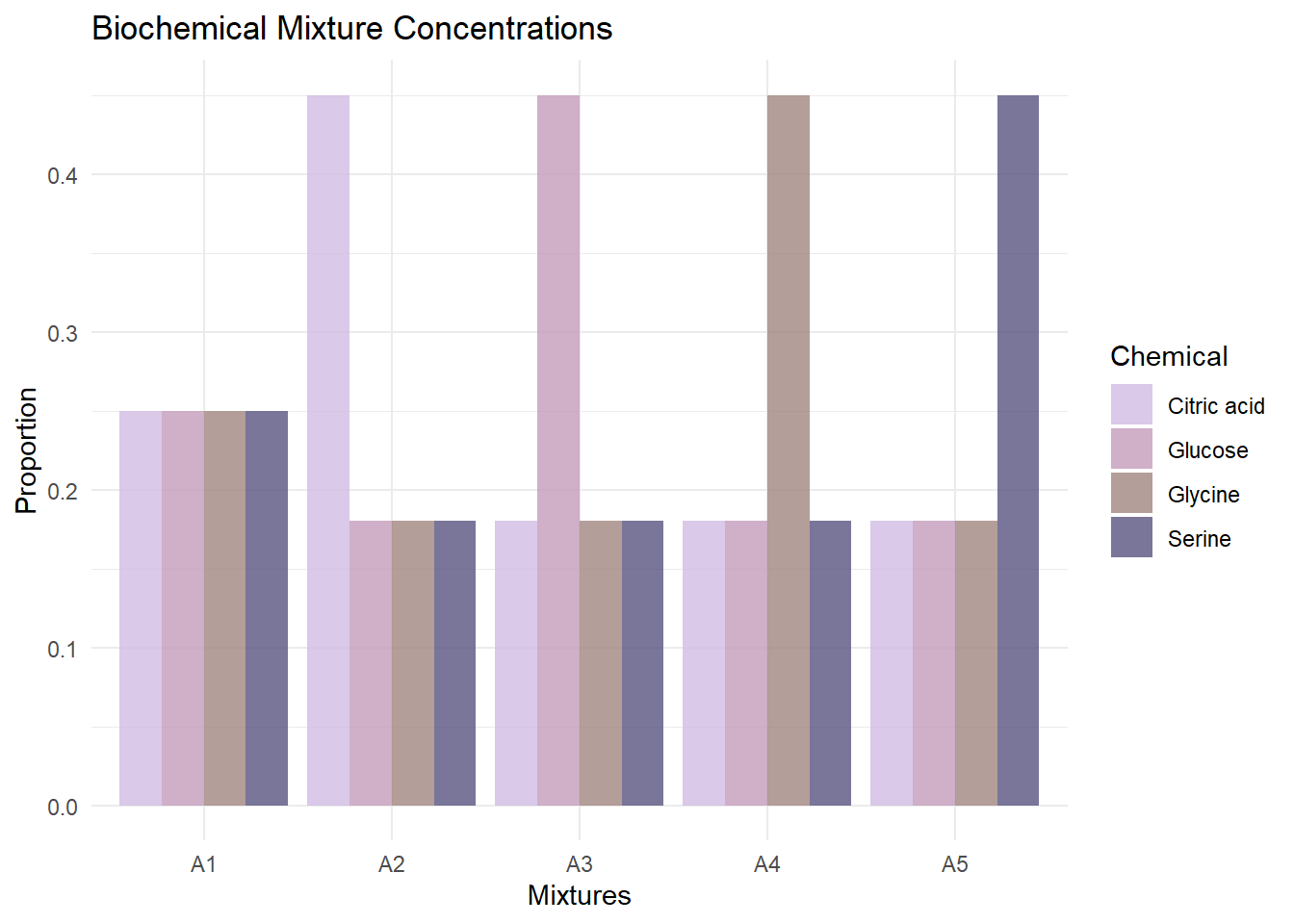
Pure Component Spectra
We use the Raman spectra of the dissolved biochemicals:
pure_diss_df <- read.csv(file.path(data_dir, "4BasesLiquid_CA-Glu-Gly-Ser.csv"), header = FALSE)
titles <- c("Citric acid", "Glucose", "Glycine", "Serine")
plot_list <- vector("list", 4)

for (i in 1:4) {
  spectrum_data <- t(pure_diss_df[i,]) |> as.data.frame()
  colnames(spectrum_data) <- c("Intensity")
  spectrum_data$RamanShift <- 1:ncol(pure_diss_df)

  plot_list[[i]] <- ggplot(spectrum_data, aes(x = RamanShift, y = Intensity)) +
    geom_line(color = "darkgreen", linewidth = 0.7) +
    labs(title = titles[i], x = "Raman Shift (index)", y = "Intensity") +
    theme_minimal()
}

grid.arrange(grobs = plot_list, ncol = 2)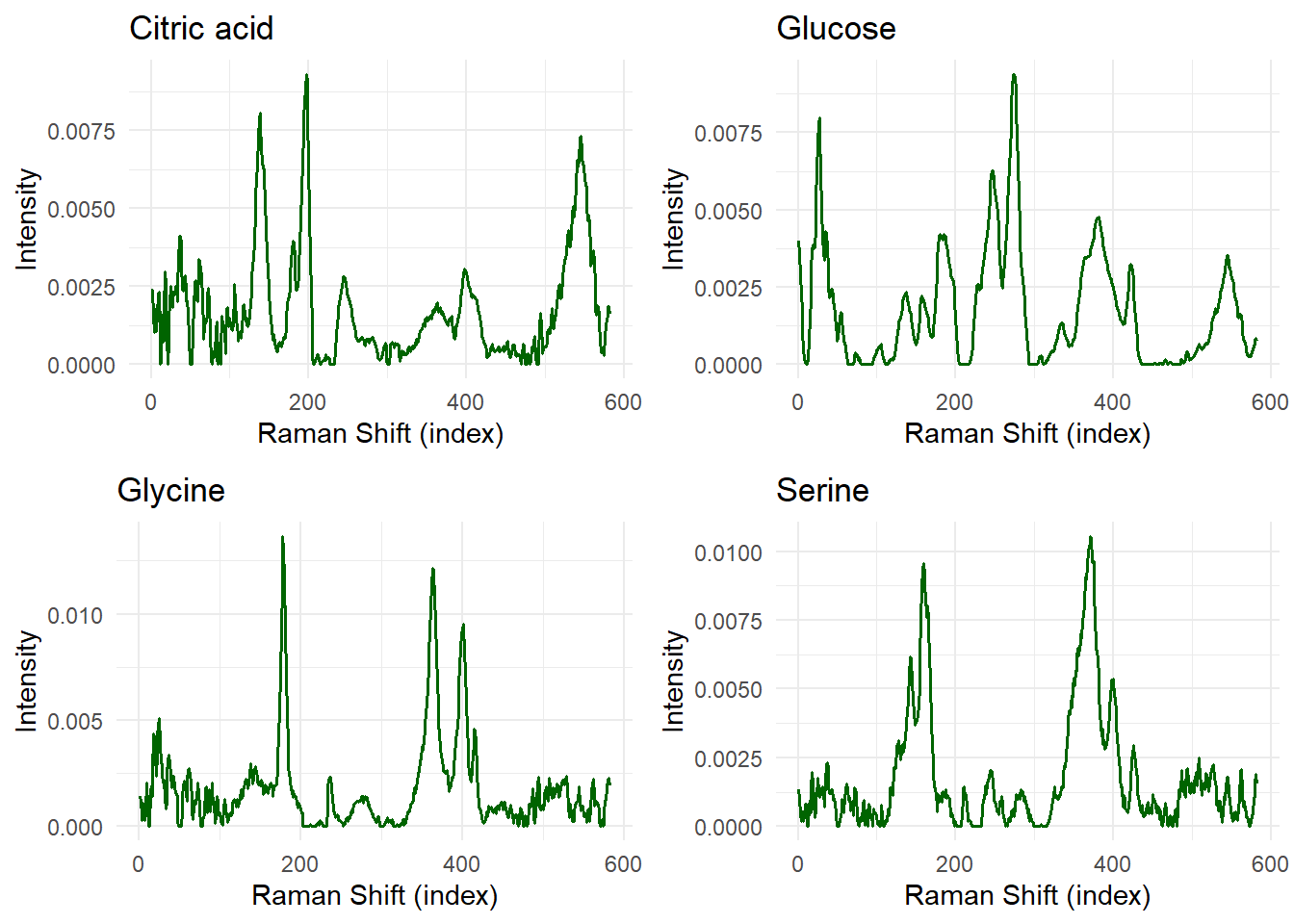
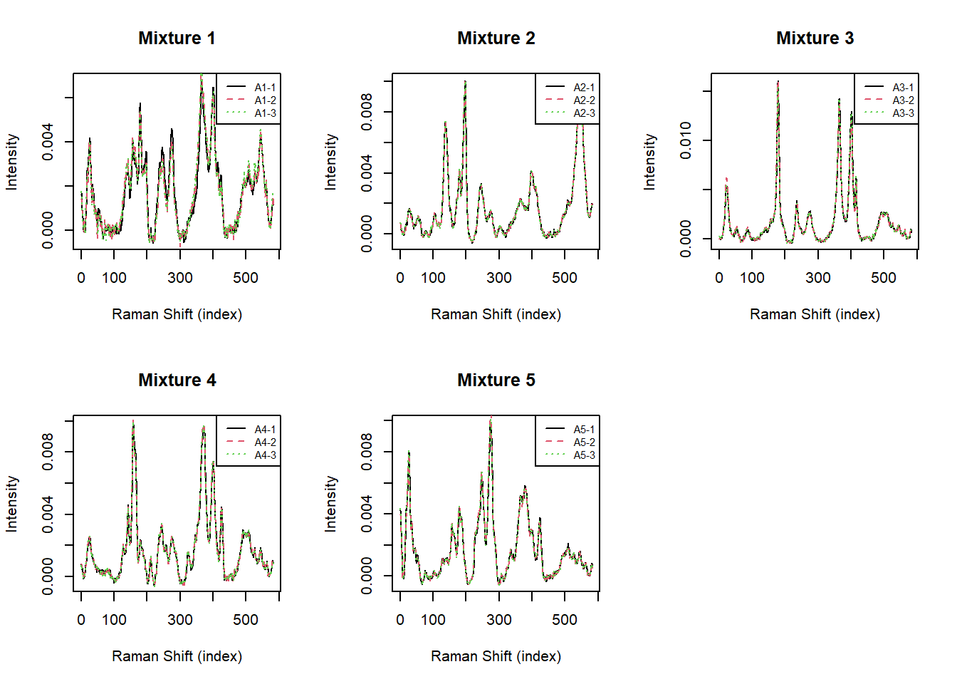
Observed Mixture Data
The data we analyze consists of 3 replicates of the 5 mixtures (15 total observations):
misc_gbrnmf <- read.csv(file.path(data_dir, "nmf_data_CA_Glu_Gly_Ser.csv"), header = FALSE)
head(misc_gbrnmf[, 1:6])
V1 V2 V3 V4 V5 V6
1 0.0016324002 0.0016879409 0.0009353232 6.744077e-04 0.0005896238 4.254590e-04
2 0.0014378929 0.0013663762 0.0010029572 6.696975e-04 0.0004860160 3.062998e-04
3 0.0017927613 0.0014456128 0.0010740219 7.397337e-04 0.0003225643 2.987971e-04
4 0.0006090482 0.0005901997 0.0002831880 1.599110e-04 0.0001392164 1.633525e-04
5 0.0007106174 0.0004973362 0.0004058312 7.522834e-05 0.0002139933 1.035101e-06
6 0.0007349224 0.0006671383 0.0005839417 2.905072e-04 0.0001725518 1.030777e-04Let’s visualize the Raman spectra we will need to unmix for each mixture:
par(mfrow = c(2, 3))
titles_mix <- sapply(1:5, function(i) paste0("A", i, "-", 1:3)) |> as.vector()

for (j in c(1, 4, 7, 10, 13)) {
  plot(1:length(misc_gbrnmf[j,]), as.numeric(misc_gbrnmf[j,]),
       type = "l", ylab = "Intensity", xlab = "Raman Shift (index)",
       col = 1, lty = 1, main = paste("Mixture", ceiling(j/3)))
  for (i in (j+1):(j+2)) {
    lines(1:length(misc_gbrnmf[i,]), as.numeric(misc_gbrnmf[i,]),
          col = i - j + 1, lty = i - j + 1)
  }
  legend("topright", legend = titles_mix[j:(j+2)], col = 1:3, lty = 1:3, cex = 0.7)
}
GBR-NMF Initialization
Before running BPSS, we use GBR-NMF to obtain initial estimates. This is crucial because BPSS solutions are not unique, and good initialization helps the MCMC sampler converge to meaningful solutions.
bases <- matrix(c(
  as.numeric(pure_diss_df[1, ]),
  as.numeric(pure_diss_df[2, ]),
  as.numeric(pure_diss_df[3, ]),
  as.numeric(pure_diss_df[4, ])
), nrow = 4, ncol = ncol(pure_diss_df), byrow = TRUE)

mat <- as.matrix(misc_gbrnmf[c(1, 4, 7, 10, 13), ])
mat <- t(apply(mat, 1, scale_row_S))

nmf.out <- cnmf(mat, maxit = 10000, q = 4, s = bases)

w <- nmf.out$w
a <- nmf.out$a
s <- nmf.out$s
The way GBR-NMF works is by setting component signals as constant and estimating their concentrations. Since our method is initialized at this solution, but allows component signals to vary, we can interpret our model as a probabilistic version of GBR-NMF.
Setting Up BPSS Priors
We use the GBR-NMF results to inform our priors. Specifically, we set the expectation of each random variable to its corresponding GBR-NMF value, with variance set to 0.01.
E <- 1 * 10^-3

wa <- w %*% a

# Normalize each row (mixture) to sum to 1
wa <- t(apply(wa, 1, scale_row_A))

# Ensure values are within truncation bounds [0.001, 1.001]
wa <- pmax(pmin(wa, 1.001), 0.001)

s <- t(apply(s, 1, scale_row_S)) + E

# Ensure s values are within truncation bounds [0.001, 1.001]
s <- pmax(pmin(s, 1.001), 0.001)

mat <- t(apply(mat, 1, scale_row_S)) + E

s_expects <- s
a_expects <- wa

var <- 0.01

alpha_a <- a_expects^2 / var
beta_a <- a_expects / var

lambda_s <- 1 / s_expects

alpha_a[alpha_a == 0 | is.na(alpha_a)] <- E
beta_a[beta_a == 0 | is.na(beta_a)] <- E
lambda_s[lambda_s == 0 | is.infinite(lambda_s) | is.na(lambda_s)] <- E

p <- 4
m <- nrow(mat)
n <- ncol(mat)
Running the Gibbs Sampler
Now we can run our MCMC sampler.
mat_jags <- mat

data.list <- list(
  X = mat_jags,
  m = m,
  n = n,
  p = p,
  E = E,
  lambda_s = lambda_s,
  alpha_a = alpha_a,
  beta_a = beta_a
)

params <- c("A", "S")

inits1 <- dump.format(list(
  A = wa,
  S = s,
  .RNG.name = "base::Wichmann-Hill",
  .RNG.seed = 87460945
))

inits2 <- dump.format(list(
  A = wa,
  S = s,
  .RNG.name = "base::Marsaglia-Multicarry",
  .RNG.seed = 874609
))

inits3 <- dump.format(list(
  A = wa,
  S = s,
  .RNG.name = "base::Super-Duper",
  .RNG.seed = 8746
))

inits4 <- dump.format(list(
  A = wa,
  S = s,
  .RNG.name = "base::Mersenne-Twister",
  .RNG.seed = 874
))

posterior <- run.jags(
  model = BPSS_Gamma_Exponential,
  data = data.list,
  monitor = params,
  inits = c(inits1, inits2, inits3, inits4),
  n.chains = 4,
  adapt = 1000,
  burnin = 5000,
  sample = 5000,
  thin = 10,
  method = "parallel"
)
Calling 4 simulations using the parallel method...
Following the progress of chain 1 (the program will wait for all chains
to finish before continuing):
Welcome to JAGS 4.3.1 on Tue Nov 18 14:58:51 2025
JAGS is free software and comes with ABSOLUTELY NO WARRANTY
Loading module: basemod: ok
Loading module: bugs: ok
. . Reading data file data.txt
. Compiling model graph
Resolving undeclared variables
Allocating nodes
Graph information:
Observed stochastic nodes: 5278
Unobserved stochastic nodes: 2353
Total graph size: 11135
. Reading parameter file inits1.txt
. Initializing model
. Adapting 1000
-------------------------------------------------| 1000
++++++++++++++++++++++++++++++++++++++++++++++++++ 100%
Adaptation successful
. Updating 5000
-------------------------------------------------| 5000
************************************************** 100%
. . . Updating 50000
-------------------------------------------------| 50000
************************************************** 100%
. . . . Updating 0
. Deleting model
.
All chains have finished
Simulation complete. Reading coda files...
Coda files loaded successfully
Note: Summary statistics were not produced as there are >50 monitored
variables
[To override this behaviour see ?add.summary and ?runjags.options]
FALSEFinished running the simulationAS <- as.mcmc.list(posterior)[[1]] |> as.data.frame()
for (i in 2:4) {
AS <- rbind(AS, as.mcmc.list(posterior)[[i]] |> as.data.frame())
}
A <- AS[, grep("^A\\[", names(AS))]
S <- AS[, grep("^S\\[", names(AS))]Results
Recovered Pure Spectra with Uncertainty
res <- get_plots_95_ci_spec(4, S, "median", 4)
wavelength <- 1:ncol(mat)

g1 <- plot_95_ci_spec(res, wavelength, 1)
g2 <- plot_95_ci_spec(res, wavelength, 2)
g3 <- plot_95_ci_spec(res, wavelength, 3)
g4 <- plot_95_ci_spec(res, wavelength, 4)

grid.arrange(g1, g2, g3, g4, nrow = 2, ncol = 2)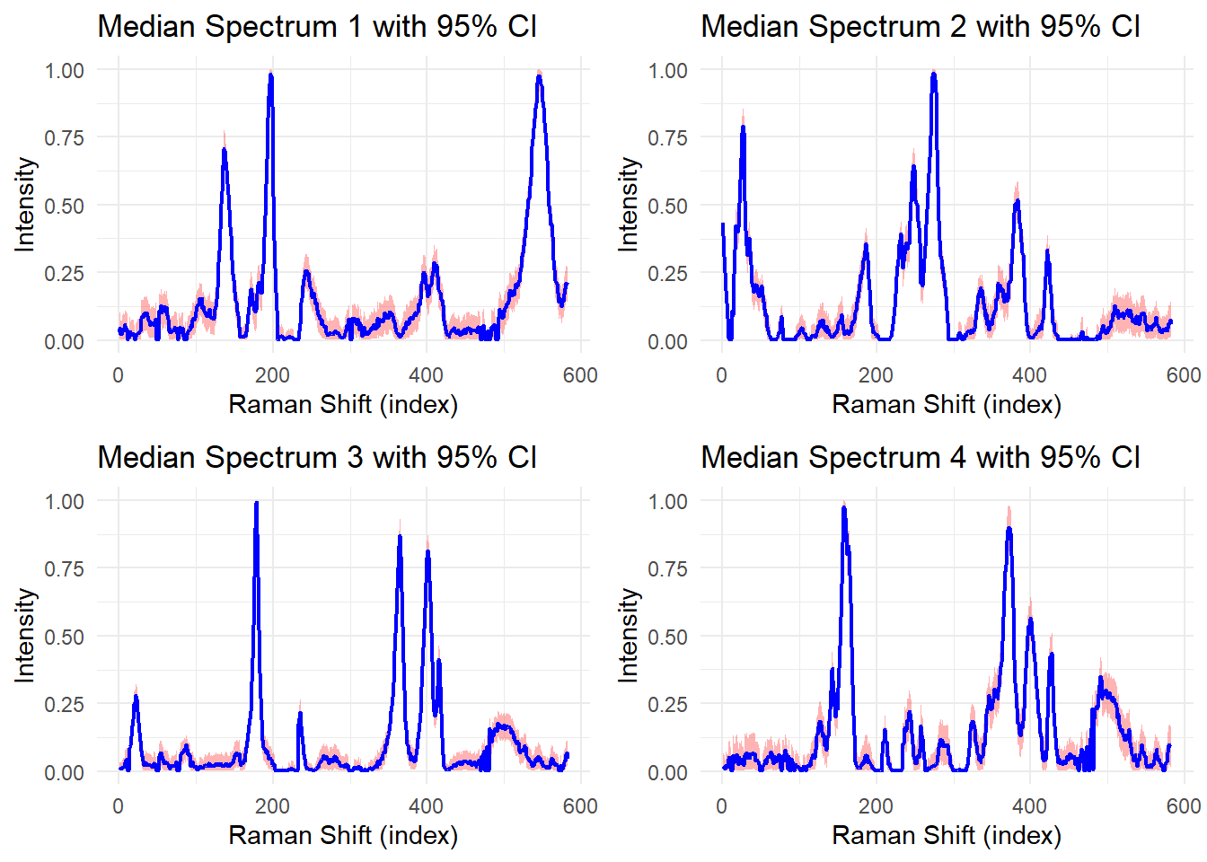
The blue lines show the median estimates of the recovered pure spectra, while the red shaded regions represent 95% credible intervals. Narrow intervals indicate high confidence in the recovered spectra, while wide intervals suggest greater uncertainty.
Recovered Mixing Proportions
Let’s examine the posterior distributions of the mixing coefficients for the first mixture:
A_list <- get_A_values_and_median(A, n = m, "median")

g1 <- get_plots_A_hist(A_list, 1)
g2 <- get_plots_A_hist(A_list, 2)
g3 <- get_plots_A_hist(A_list, 3)
g4 <- get_plots_A_hist(A_list, 4)

grid.arrange(g1, g2, g3, g4, nrow = 2, ncol = 2)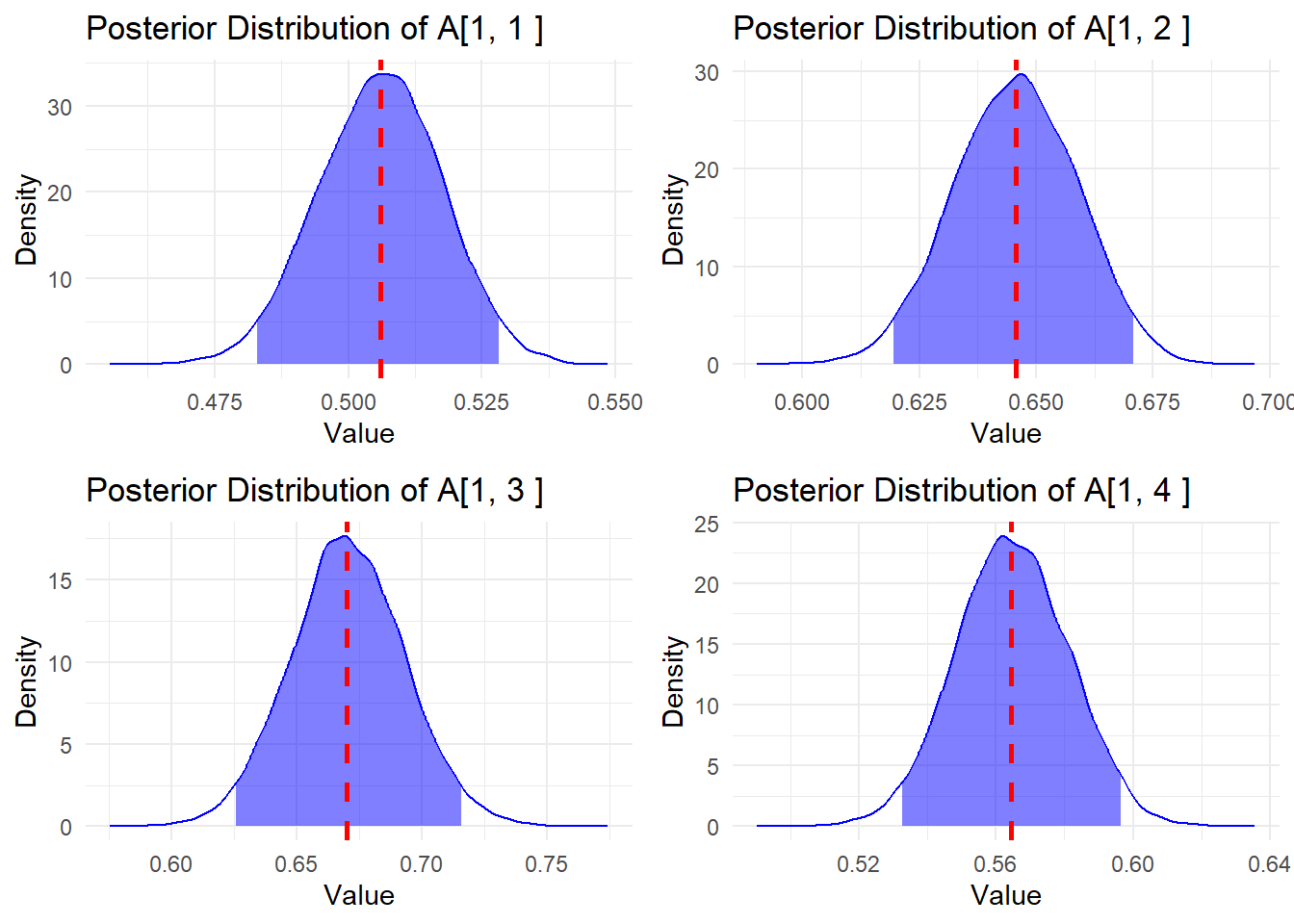
The red dashed line shows the median estimate, and the blue shaded area represents the 95% credible interval.
Discussion
With this, we have come up with a probabilstic version of GBR-NMF! So why do we want to do this? Well, there are a two main reasons:
Uncertainty Quantification: Unlike point estimates from GBR-NMF, BPSS provides full posterior distributions, allowing us to quantify uncertainty in both the recovered spectra and mixing proportions.
Pure Components Can Change: By degault GBR-NMF does not allow the pure components to change, but BPSS does. This is important because in reality, the pure components of a chemical can change depending on the conditions of the experiment such as temperature, pressure, and solvent.
If you would like to read more about the advantages of BPSS, you can read my undergraduate honours thesis here https://open.library.ubc.ca/soa/cIRcle/collections/undergraduateresearch/52966/items/1.0443983.
References
Brie, David, Saı̈d Moussaoui, Sebastian Miron, Cédric Carteret, and Manuel Dossot. 2016. “Bayesian Positive Source Separation for Spectral Mixture Analysis.” In Data Handling in Science and Technology, 30:279–309. Elsevier.
Milligan, Kirsty, Kendra Scarrott, Jeffrey L Andrews, Alexandre G Brolo, Julian J Lum, and Andrew Jirasek. 2023. “Reconstruction of Raman Spectra of Biochemical Mixtures Using Group and Basis Restricted Non-Negative Matrix Factorization.” Applied Spectroscopy 77 (7): 698–709.
Shreeves, Phillip, Jeffrey L Andrews, Xinchen Deng, Ramie Ali-Adeeb, and Andrew Jirasek. 2023. “Nonnegative Matrix Factorization with Group and Basis Restrictions.” Statistics in Biosciences 15 (3): 608–32.